Position-dependent photon fields / 2 - Propagating through a spatially-scaled photon field

Notebook 1 generated and verified the \(1/r\)-scaled PowerlawPhotonField. Here that field is put to use: a power-law gamma-ray beam is propagated through the homogeneous and the :math:`1/r`-scaled field, and the surviving spectra are compared with a simple analytic reference. A final section checks how the result converges as the spatial grid is refined.

Geometry

One-dimensional. The source sits at \(x=+5\) kpc and emits in the \(-x\) direction; Observer1D detects at \(x=0\), so every photon crosses the column \([0,5]\) kpc. The runs are absorption-only: EMPairProduction is added with haveElectrons=False, and an ObserverElectronVeto discards any \(e^\pm\), so a photon is simply removed when it pair-produces. The scaled field is less dense, absorbs less, and so its cutoff lies at higher energy than the homogeneous one.

Step size matters. EMPairProduction freezes the interaction rate at the start of each step, so for a spatially varying field the step must be small compared with \(r_s=0.2\) kpc; MAX_STEP = 0.01 kpc is used throughout.

Setup

Constants, the scaling profile, the per-node field writers, the generate_spatial_field helper and a few analysis utilities. The on-disk conventions (filename coordinates, reversed energy/density ordering) are explained in notebook 1; the writers are repeated here so this notebook is self-contained. The base tables (PowerlawPhotonField) must already exist in the share folder — run notebook 1 first.

from pathlib import Path

import crpropa as crp
import matplotlib.pyplot as plt
import numpy as np
from crpropa import GeV, MeV, Output, PeV, Vector3d, eV, kpc

# share folder this CRPropa build reads its tables from
CRPROPA_DATA = Path(crp.getDataPath(""))
BASE_FIELD = "PowerlawPhotonField"  # homogeneous base field (tables from notebook 1)
SPATIAL_FIELD = "PowerlawPhotonFieldTest1R"  # 1/r-scaled field (no "_" in the name)

# 1-D geometry, source and propagation
X_SRC = 5.0 * kpc  # source at +5 kpc, emits in -x, observer at x=0
E_SRC_MIN, E_SRC_MAX, SOURCE_INDEX = 10 * GeV, 10 * PeV, -1.0
E_MIN_STOP = 10 * MeV
MIN_STEP, MAX_STEP = 1e-4 * kpc, 1e-2 * kpc  # step must resolve r_s = 0.2 kpc

# analysis binning
N_EVENTS = 100_000
E_MIN_EV, E_MAX_EV, N_BINS = 1e10, 1e16, 60
bins = np.logspace(np.log10(E_MIN_EV), np.log10(E_MAX_EV), N_BINS + 1)
centers = np.sqrt(bins[:-1] * bins[1:])


def f_soft_1_over_r(x, y=0.0, z=0.0, A=1.0, r_s=0.2):
    """Softened central scaling f(0)=1, falling outward as r_s / (r + r_s)."""
    r = np.sqrt(x * x + y * y + z * z)
    return A * r_s / (r + r_s)

Per-node field writers

generate_spatial_field writes one file per grid node, each scaled by \(f\) (see notebook 1 for the on-disk format). The fields are written into the share folder and kept there.

def node_suffix(x, y, z):
    # store -x: the reader reconstructs the coordinate from the filename
    return f"node_{-x:.8g}_{y:.8g}_{z:.8g}"


def _data_lines(path):
    return [l for l in open(path) if l.strip() and not l.lstrip().startswith("#")]


def _write_reversed(src, dst, scale=1.0):
    """Energy/density: reverse line order; optionally scale every column."""
    with open(dst, "w") as f:
        for line in reversed(_data_lines(src)):
            f.write(" ".join(f"{float(v) * scale:.16e}" for v in line.split()) + "\n")


def _scale_rate_like(src, dst, scale):
    """Rate/CDF: keep order and header; scale all columns except the first."""
    seen = False
    with open(src) as fin, open(dst, "w") as fout:
        for line in fin:
            s = line.strip()
            if not s or s.startswith("#"):
                fout.write(line)
                continue
            p = s.split()
            if not seen and len(p) > 2:  # CDF s-grid row: keep unchanged
                fout.write(line)
                seen = True
                continue
            seen = True
            fout.write(
                p[0] + " " + " ".join(f"{float(v) * scale:.16e}" for v in p[1:]) + "\n"
            )


def generate_spatial_field(name, n_nodes=21):
    """Write the 1/r-scaled field with n_nodes nodes over x in [-5, 5] kpc."""
    assert "_" not in name
    be = CRPROPA_DATA / "Scaling" / f"{BASE_FIELD}_photonEnergy.txt"
    bd = CRPROPA_DATA / "Scaling" / f"{BASE_FIELD}_photonDensity.txt"
    br = CRPROPA_DATA / "EMPairProduction" / f"rate_{BASE_FIELD}.txt"
    bc = CRPROPA_DATA / "EMPairProduction" / f"cdf_{BASE_FIELD}.txt"
    oe = CRPROPA_DATA / "Scaling" / name / "photonEnergy"
    od = CRPROPA_DATA / "Scaling" / name / "photonDensity"
    orr = CRPROPA_DATA / "EMPairProduction" / name / "Rate"
    oc = CRPROPA_DATA / "EMPairProduction" / name / "CumulativeRate"
    for d in (oe, od, orr, oc):
        d.mkdir(parents=True, exist_ok=True)
    for x in np.linspace(-5, 5, n_nodes):
        f = f_soft_1_over_r(x)
        suf = node_suffix(x, 0.0, 0.0)
        _write_reversed(be, oe / f"{name}_{suf}.txt")
        _write_reversed(bd, od / f"{name}_{suf}.txt", scale=f)
        _scale_rate_like(br, orr / f"rate_{name}_{suf}.txt", f)
        _scale_rate_like(bc, oc / f"cdf_{name}_{suf}.txt", f)


generate_spatial_field(SPATIAL_FIELD)
print("generated", SPATIAL_FIELD)

generated PowerlawPhotonFieldTest1R

Analysis helpers

binned_spectrum reads a CRPropa Event1D output and histograms it into counts per \(\Delta\log_{10}E\); base_rate interpolates the homogeneous pair-production rate.

def binned_spectrum(path):
    """Surviving counts per dlog10E from a CRPropa Event1D output file."""
    d = np.genfromtxt(path, names=True)
    counts, _ = np.histogram(d["E"], bins=bins, weights=d["W"])
    return counts / np.diff(np.log10(bins))


def base_rate(E_eV):
    """Homogeneous pair-production rate [1/Mpc] interpolated at E_eV."""
    t = np.genfromtxt(
        CRPROPA_DATA / "EMPairProduction" / f"rate_{BASE_FIELD}.txt", comments="#"
    )
    return np.interp(np.log10(E_eV), t[:, 0], t[:, 1], left=0.0, right=0.0)

1. Surviving spectrum: homogeneous vs \(1/r\)-scaled

run_spectrum propagates the power-law beam through a given field and saves the survivors. It is called once for the homogeneous TabularPhotonField (written to events_homogeneous.txt) and once for the TabularSpatialPhotonField (events_1r.txt); both files are kept for inspection or re-use.

def run_spectrum(field, output_file, n=N_EVENTS):
    """Propagate the power-law beam through `field`, saving the survivors to `output_file`."""
    sim = crp.ModuleList()
    sim.add(crp.SimplePropagation(MIN_STEP, MAX_STEP))  # bounded step (resolves r_s)
    sim.add(crp.EMPairProduction(field, False, 0.0))  # absorption only, no e+- produced
    sim.add(crp.MinimumEnergy(E_MIN_STOP))
    sim.add(crp.MaximumTrajectoryLength(20 * kpc))

    obs = crp.Observer()
    obs.add(crp.Observer1D())
    obs.add(crp.ObserverElectronVeto())  # we are only interested in photons
    output = crp.TextOutput(output_file, Output.Event1D)
    output.setEnergyScale(eV)
    output.enable(output.WeightColumn)
    output.disable(output.CandidateTagColumn)  # not needed in this analysis
    obs.onDetection(output)
    sim.add(obs)

    source = crp.Source()
    source.add(crp.SourcePosition(Vector3d(X_SRC, 0, 0)))
    source.add(crp.SourceDirection(Vector3d(-1, 0, 0)))
    source.add(crp.SourceParticleType(22))
    source.add(crp.SourcePowerLawSpectrum(E_SRC_MIN, E_SRC_MAX, SOURCE_INDEX))
    sim.run(source, n, True)
    output.close()


run_spectrum(crp.TabularPhotonField(BASE_FIELD, False), "events_homogeneous.txt")
run_spectrum(crp.TabularSpatialPhotonField(SPATIAL_FIELD), "events_1r.txt")
print("done")

crpropa::ModuleList: Number of Threads: 8
crpropa::ModuleList: Number of Threads: 8
done

Bin both runs and build the analytic reference. The column traversed shrinks from \(L_0=5\) kpc (homogeneous) to \(L_s=\int_0^5 f\,\mathrm{d}x\) (scaled); the flat injection normalisation is \(\mathrm{norm}=N/\log_{10}(E_{\max}/E_{\min})\).

spec_unscaled = binned_spectrum("events_homogeneous.txt")
spec_scaled = binned_spectrum("events_1r.txt")

x = np.linspace(0, 5, 5000)
L0 = 5.0 / 1000.0  # homogeneous column [Mpc]
Ls = np.trapezoid(f_soft_1_over_r(x), x) / 1000.0  # 1/r-scaled column [Mpc]
norm = N_EVENTS / np.log10(E_MAX_EV / E_MIN_EV)  # flat counts / dlog10E for index -1
rate_c = base_rate(centers)
spec_ref_unscaled = norm * np.exp(-rate_c * L0)
spec_ref_scaled = norm * np.exp(-rate_c * Ls)
print(f"mean scaling <f> = Ls / L0 = {Ls / L0:.3f}")

mean scaling <f> = Ls / L0 = 0.130

fig, (ax, axr) = plt.subplots(
    2, 1, figsize=(7, 6), sharex=True, gridspec_kw={"height_ratios": [2.5, 1]}
)
ax.step(centers, spec_unscaled, where="mid", color="C0", label="homogeneous (sim)")
ax.step(centers, spec_scaled, where="mid", color="C1", label="1/r-scaled (sim)")
ax.plot(centers, spec_ref_unscaled, "C0--", lw=1, label="homogeneous (analytic)")
ax.plot(centers, spec_ref_scaled, "C1--", lw=1, label="1/r-scaled (analytic)")
ax.set_yscale("log")
ax.set_ylim(3e1, 1.3 * norm)
ax.set_ylabel(r"counts / $\Delta\log_{10}E$")
ax.set_title("Surviving spectrum: homogeneous vs 1/r-scaled field")
ax.legend(fontsize=8)

with np.errstate(divide="ignore", invalid="ignore"):
    axr.step(
        centers,
        np.where(spec_ref_scaled > 0, spec_scaled / spec_ref_scaled, np.nan),
        where="mid",
        color="C1",
    )
axr.axhline(1, color="k", ls="--", lw=0.8)
axr.set_xscale("log")
axr.set_xlim(1e10, 1e13)  # survivors cut off well below the 10 PeV injection ceiling
axr.set_ylim(0.5, 1.5)
axr.set_ylabel("sim / analytic")
axr.set_xlabel(r"$E_\gamma$ [eV]")
plt.tight_layout()
plt.show()

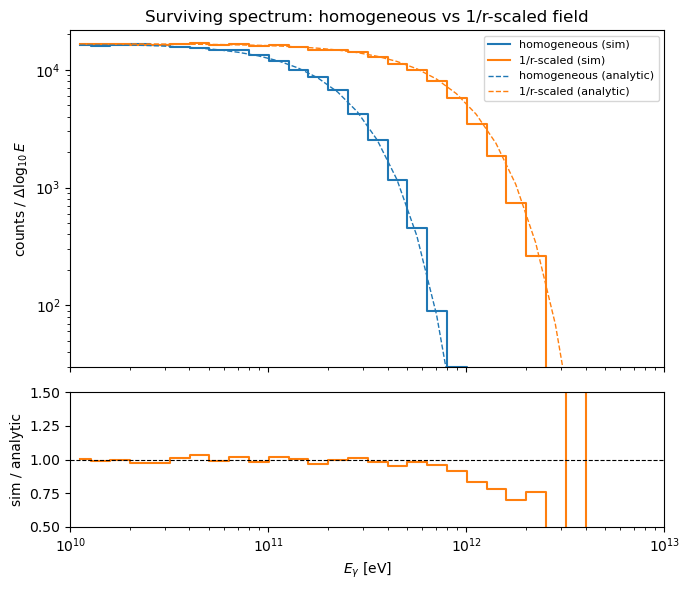
The scaled field absorbs less, so its cutoff sits about a decade higher than the homogeneous one, and the simulation tracks the analytic reference across the turnover. The tail is noisy at this N_EVENTS; raise it for a publication-quality figure.

2. Convergence with grid sampling

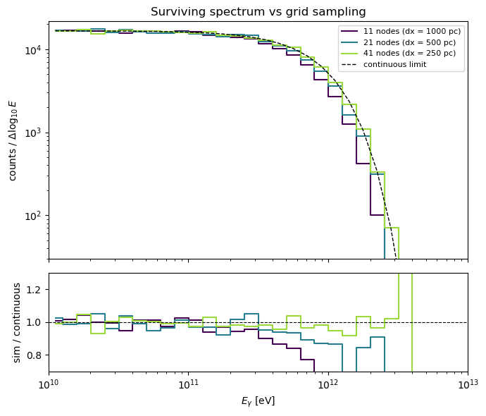
The spatial rate is taken from the nearest node, so a coarse grid mis-resolves the steep central region. The same beam is propagated through the \(1/r\) field generated at several samplings and compared with the continuous-field reference from section 1. Each grid and its event file (events_grid<N>.txt) are kept on disk.

GRID_SIZES = [11, 21, 41]

specs = {}
for n_nodes in GRID_SIZES:
    name = f"PowerlawGrid{n_nodes}"
    generate_spatial_field(name, n_nodes)
    run_spectrum(crp.TabularSpatialPhotonField(name), f"events_grid{n_nodes}.txt")
    specs[n_nodes] = binned_spectrum(f"events_grid{n_nodes}.txt")
print("done")

crpropa::ModuleList: Number of Threads: 8
crpropa::ModuleList: Number of Threads: 8
crpropa::ModuleList: Number of Threads: 8
done

fig, (ax, axr) = plt.subplots(
    2, 1, figsize=(7, 6), sharex=True, gridspec_kw={"height_ratios": [2.4, 1]}
)
colors = plt.cm.viridis(np.linspace(0, 0.85, len(GRID_SIZES)))
for color, n_nodes in zip(colors, GRID_SIZES):
    dx = 10000 / (n_nodes - 1)  # node spacing [pc]
    ax.step(
        centers,
        specs[n_nodes],
        where="mid",
        color=color,
        label=f"{n_nodes} nodes (dx = {dx:.0f} pc)",
    )
    with np.errstate(divide="ignore", invalid="ignore"):
        axr.step(
            centers,
            np.where(spec_ref_scaled > 0, specs[n_nodes] / spec_ref_scaled, np.nan),
            where="mid",
            color=color,
        )
ax.plot(centers, spec_ref_scaled, "k--", lw=1, label="continuous limit")
ax.set_xscale("log")
ax.set_yscale("log")
ax.set_ylim(3e1, 1.3 * norm)
ax.set_ylabel(r"counts / $\Delta\log_{10}E$")
ax.set_title("Surviving spectrum vs grid sampling")
ax.legend(fontsize=8)

axr.axhline(1, color="k", ls="--", lw=0.8)
axr.set_xscale("log")
axr.set_xlim(1e10, 1e13)  # survivors cut off well below the 10 PeV injection ceiling
axr.set_ylim(0.7, 1.3)
axr.set_ylabel("sim / continuous")
axr.set_xlabel(r"$E_\gamma$ [eV]")
plt.tight_layout()
plt.show()

3. Notes

• The samplings overlap and track the continuous limit through the turnover; the coarsest grid deviates most near the cutoff. For this smooth \(1/r\) profile even 11 nodes is only modestly off — a sharper profile, or a grid that misses the central peak, would widen the spread.

• The propagation step must stay well below \(r_s\) (here MAX_STEP = 0.01 kpc), since EMPairProduction freezes the rate over each step.