Position-dependent photon fields / 1 - Generating a spatially-scaled power-law photon field

This notebook extends the custom-photon-field example (doc/pages/example_notebooks/custom_photonfield/custom-photon-field.ipynb) to a position-dependent photon field. It first reproduces the homogeneous PowerlawPhotonField from that example, then modulates it in space with a softened \(1/r\) profile and verifies the result.

As in the custom-photon-field example, two photon-field classes are involved for every model: one that lives in the CRPropa-data repository and produces the tabulated files (interaction rates, densities), and one that lives in CRPropa and is used during propagation. Here the second class is the built-in TabularSpatialPhotonField.

Physics background

High-energy photons are attenuated by pair production on the soft radiation field, \(\gamma + \gamma_{\rm bg} \to e^+ e^-\). Its kinematic threshold \(E_\gamma\,\epsilon \gtrsim (m_e c^2)^2\) means that for the target field used here (\(\epsilon\) up to \(\sim 10^3\) eV) absorption switches on around a TeV.

The Galactic interstellar radiation field is concentrated toward the Galactic centre and the disk, so the attenuation depends on where the photon is, not only on its energy. TabularSpatialPhotonField captures this by storing one comoving density spectrum \(\mathrm{d}n/\mathrm{d}\epsilon\) [1/m³/J] per spatial grid node; a query returns the nearest node’s spectrum, interpolated in energy. The redshift dependence is dropped, since the application is Galactic.

Setup

The CRPropa-data repository provides the base classes (photonField) and the table generators (calc_all). Set crpropa_data_path below to your local CRPropa-data checkout. The share folder is taken from crp.getDataPath(""), so the tables generated here are written exactly where CRPropa reads them during propagation.

import subprocess
import sys
import warnings
from pathlib import Path

import crpropa as crp
import numpy as np
from crpropa import TeV, Vector3d, ccm, eV, kpc

# path to the local CRPropa-data repository checkout (adjust to your installation)
crpropa_data_path = "..."
# share folder this CRPropa build reads its tables from; derived automatically so the
# tables generated below land exactly where propagation looks them up.
crpropa_share_path = crp.getDataPath("")
sys.path.append(crpropa_data_path)

import matplotlib.pyplot as plt

import calc_all as ca  # CRPropa-data: interaction-table generators
import photonField as pf  # CRPropa-data: base photon-field classes

1. Define the homogeneous photon field (CRPropa-data)

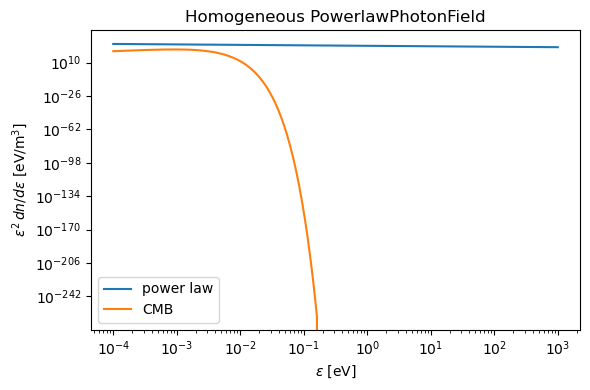
The starting point is the single power law with exponential cutoffs from the custom-photon-field example, \(\mathrm{d}n/\mathrm{d}\epsilon \propto (\epsilon/\mathrm{eV})^{\alpha}\) on \([\epsilon_{\min},\epsilon_{\max}]\). The class below is taken verbatim from that example; it inherits from the CRPropa-data base class and provides the mandatory name, info, redshift, the energy grid, the density, and getDensity/getEmin/getEmax.

class PowerlawPhotonField(pf.PhotonField):

    def __init__(self, norm=1e28, slope=-2.5, eMin=1e-4 * eV, eMax=1e3 * eV):
        """Power law with exponential cutoffs; norm is n(eps = 1 eV)."""
        super(PowerlawPhotonField, self).__init__()
        self.name = "PowerlawPhotonField"
        self.info = (
            "Single power law photon field with exponential cutoffs at both ends."
        )
        self.redshift = None
        self.norm = norm
        self.slope = slope
        self.eMin = eMin
        self.eMax = eMax
        self.energy = np.logspace(np.log10(self.eMin), np.log10(self.eMax), 101) / eV
        self.photonDensity = self.getDensity(self.energy * eV) / (eV**-1 * ccm**-1)

    def getDensity(self, eps, z=0):
        """Comoving spectral number density dn/deps [1/m^3/J] at energy eps [J]."""
        if type(eps) == np.ndarray:
            return np.array([self.getDensity(_eps, z) for _eps in eps])
        if (eps >= self.eMin) & (eps <= self.eMax):
            return self.norm * (eps / eV) ** self.slope
        else:
            return 0.0

    def getEmin(self):
        return self.eMin

    def getEmax(self):
        return self.eMax


field = PowerlawPhotonField()
print("field :", field.name)
print("range :", f"{field.getEmin()/eV:.1e} .. {field.getEmax()/eV:.1e} eV")

field : PowerlawPhotonField
range : 1.0e-04 .. 1.0e+03 eV

Plot the field

The power-law field is shown as \(\epsilon^2\,\mathrm{d}n/\mathrm{d}\epsilon\), with the cosmic microwave background for comparison (as in the custom-photon-field example).

field_cmb = pf.CMB()
eps = np.logspace(-4, 3, 300) * eV
c = eps**2 / eV**2
plt.figure(figsize=(6, 4))
plt.plot(eps / eV, c * field.getDensity(eps), label="power law")
plt.plot(eps / eV, c * field_cmb.getDensity(eps), label="CMB")
plt.loglog()
plt.legend()
plt.xlabel(r"$\epsilon$ [eV]")
plt.ylabel(r"$\epsilon^2\,dn/d\epsilon$ [eV/m$^3$]")
plt.title("Homogeneous PowerlawPhotonField")
plt.tight_layout()
plt.show()

/home/grindegreen/miniconda3/envs/crpropa-position/CRPropa3-data/photonField.py:79: RuntimeWarning: overflow encountered in expm1
  return 8*np.pi / c_light**3 / h_planck**3 * eps**2 / np.expm1(eps / (k_boltzmann * self.T_CMB))

2. Generate the interaction tables (CRPropa-data)

calc_all precomputes the tables for all photon-dependent processes. This step is expensive (~15 minutes). It writes into ./data, which is then copied into the CRPropa share folder. The cell is guarded so it only runs if the base tables are not already present; delete the guard to force a regeneration.

base_present = (
    Path(crpropa_share_path, "Scaling", f"{field.name}_photonEnergy.txt").exists()
    and Path(crpropa_share_path, "EMPairProduction", f"rate_{field.name}.txt").exists()
)

if base_present:
    print(
        "Base tables already present in the share folder; skipping the (~15 min) generation."
    )
else:
    # 2. generate the tables
    with warnings.catch_warnings():  # density ~ 0 outside the band -> divide-by-zero warnings
        warnings.simplefilter("ignore")
        ca.EM_processes([field])
        ca.photon_fields([field])
    # 3. copy the generated tables into the share folder
    subprocess.run(["cp", "-a", "./data/.", crpropa_share_path])
    print("Generated and copied base tables for", field.name)

Base tables already present in the share folder; skipping the (~15 min) generation.

3. Scale the field in space

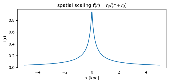
The homogeneous field is turned into a position-dependent one by multiplying its density by a softened central profile

\[f(r) = \frac{r_s}{r + r_s},\qquad r_s = 0.2\ \mathrm{kpc},\]

maximal at the centre (\(f=1\)) and falling outward. Because pair production is linear in the target photon density, the interaction rate scales by the same factor \(f\).

On-disk layout

A TabularSpatialPhotonField named NAME stores one file per grid node:

Scaling/NAME/photonEnergy/NAME_node_<-x>_<y>_<z>.txt
Scaling/NAME/photonDensity/NAME_node_<-x>_<y>_<z>.txt
EMPairProduction/NAME/Rate/rate_NAME_node_...
EMPairProduction/NAME/CumulativeRate/cdf_NAME_node_...

Two conventions are imposed by the reader and must be matched on write:

1. Coordinates are encoded in the filename, split on _; the reader applies \(x=-\,\mathrm{stod}\), so files store \(-x\). Consequently the field name must contain no ``_``, or the tokens shift.

2. Energy and density files are read reversed (each line is inserted at the front of the array, matching the high\(\to\)low ordering of the CRPropa export). The base table is stored low\(\to\)high, so it is written reversed here; after the reader reverses it again the in-memory array is increasing, as the interpolation requires. Without this, getPhotonDensity returns 0 everywhere.

SPATIAL_FIELD = "PowerlawPhotonFieldTest1R"  # no '_' in the name
assert "_" not in SPATIAL_FIELD
GRID_X_KPC = np.linspace(-5.0, 5.0, 21)  # nodes along x (odd count keeps a node at x=0)


def f_soft_1_over_r(x, y=0.0, z=0.0, A=1.0, r_s=0.2):
    r = np.sqrt(x * x + y * y + z * z)
    return A * r_s / (r + r_s)


xx = np.linspace(-5, 5, 400)
plt.figure(figsize=(6, 3))
plt.plot(xx, f_soft_1_over_r(xx))
plt.xlabel("x [kpc]")
plt.ylabel("f(r)")
plt.title(r"spatial scaling $f(r)=r_s/(r+r_s)$")
plt.tight_layout()
plt.show()

Writers

The energy and density files are written reversed; the rate and CDF files keep their order (their reader does not reverse). Every file scales by \(f\) except the energy grid.

def node_suffix(x, y, z):
    # store -x because the reader applies x = -stod(token)
    return f"node_{-x:.8g}_{y:.8g}_{z:.8g}"


def data_lines(path):
    return [l for l in open(path) if l.strip() and not l.lstrip().startswith("#")]


def write_reversed(src, dst, scale=1.0):
    """energy/density: reverse line order; optionally scale every column."""
    with open(dst, "w") as fout:
        for line in reversed(data_lines(src)):
            vals = [float(v) * scale for v in line.split()]
            fout.write(" ".join(f"{v:.16e}" for v in vals) + "\n")


def scale_rate_like(src, dst, scale):
    """rate/cdf: keep order and header; scale all columns except the first
    (log10 E, or the s-grid row of a CDF file)."""
    seen = False
    with open(src) as fin, open(dst, "w") as fout:
        for line in fin:
            s = line.strip()
            if not s or s.startswith("#"):
                fout.write(line)
                continue
            parts = s.split()
            if not seen and len(parts) > 2:  # CDF s-grid row: keep unchanged
                fout.write(line)
                seen = True
                continue
            seen = True
            rest = [float(v) * scale for v in parts[1:]]
            fout.write(parts[0] + " " + " ".join(f"{v:.16e}" for v in rest) + "\n")

4. Generate the spatial field

One file per node, scaled by f(node). The CDF files must exist (the position-dependent EMPairProduction constructor reads them) even though the absorption-only runs in the later notebooks never sample them.

DATA = Path(crpropa_share_path)
be = DATA / "Scaling" / f"{field.name}_photonEnergy.txt"
bd = DATA / "Scaling" / f"{field.name}_photonDensity.txt"
br = DATA / "EMPairProduction" / f"rate_{field.name}.txt"
bc = DATA / "EMPairProduction" / f"cdf_{field.name}.txt"

oe = DATA / "Scaling" / SPATIAL_FIELD / "photonEnergy"
od = DATA / "Scaling" / SPATIAL_FIELD / "photonDensity"
orr = DATA / "EMPairProduction" / SPATIAL_FIELD / "Rate"
oc = DATA / "EMPairProduction" / SPATIAL_FIELD / "CumulativeRate"
for d in (oe, od, orr, oc):
    d.mkdir(parents=True, exist_ok=True)

for x in GRID_X_KPC:
    f = f_soft_1_over_r(x)
    suf = node_suffix(x, 0.0, 0.0)
    write_reversed(be, oe / f"{SPATIAL_FIELD}_{suf}.txt")  # energy:  reversed, unscaled
    write_reversed(
        bd, od / f"{SPATIAL_FIELD}_{suf}.txt", scale=f
    )  # density: reversed, x f
    scale_rate_like(br, orr / f"rate_{SPATIAL_FIELD}_{suf}.txt", f)  # rate:    x f
    scale_rate_like(bc, oc / f"cdf_{SPATIAL_FIELD}_{suf}.txt", f)  # cdf:     x f

print(f"generated {len(GRID_X_KPC)} nodes for {SPATIAL_FIELD}")

generated 21 nodes for PowerlawPhotonFieldTest1R

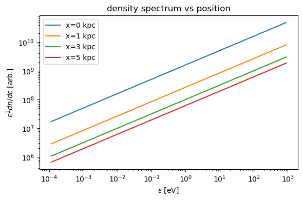
5. Check the implementation

Density gradient

The density at the centre (\(r=0\), \(f=1\)) over the density at \(r=5\) kpc should equal

\[\frac{f(0)}{f(5)}=\frac{5+r_s}{r_s}=\frac{5.2}{0.2}=26 .\]

field_sp = crp.TabularSpatialPhotonField(SPATIAL_FIELD)
Eq = 1e-20  # J, inside the band
d0 = field_sp.getPhotonDensity(Eq, 0, Vector3d(0, 0, 0))
d5 = field_sp.getPhotonDensity(Eq, 0, Vector3d(5 * kpc, 0, 0))
print(f"density(0)/density(5 kpc) = {d0/d5:.2f}  (expected {5.2/0.2:.2f})")

Eg = (
    np.logspace(
        np.log10(field_sp.getMinimumPhotonEnergy(0) / eV) + 0.05,
        np.log10(field_sp.getMaximumPhotonEnergy(0) / eV) - 0.05,
        60,
    )
    * eV
)
plt.figure(figsize=(6, 4))
for x in [0, 1, 3, 5]:
    dn = [field_sp.getPhotonDensity(e, 0, Vector3d(x * kpc, 0, 0)) for e in Eg]
    plt.loglog(Eg / eV, (Eg / eV) ** 2 * np.array(dn), label=f"x={x} kpc")
plt.xlabel(r"$\epsilon$ [eV]")
plt.ylabel(r"$\epsilon^2 dn/d\epsilon$ [arb.]")
plt.legend()
plt.title("density spectrum vs position")
plt.tight_layout()
plt.show()

density(0)/density(5 kpc) = 26.00  (expected 26.00)

Interaction rate

Passing the spatial field to EMPairProduction builds the position-dependent interaction rate (nearest-node lookup via a KD-tree). The process rate at a position should equal the base rate times \(f(r)\) of the nearest node.

rates = crp.EMPairProduction(field_sp, False, 0.0).getInteractionRates()
E = 10 * TeV
r0 = rates.getProcessRate(E, Vector3d(0, 0, 0))
print(f"{'x[kpc]':>7}{'f(r)':>9}{'rate/rate0':>12}")
for x in [0, 1, 2, 5]:
    r = rates.getProcessRate(E, Vector3d(x * kpc, 0, 0))
    print(f"{x:7.1f}{f_soft_1_over_r(x):9.4f}{r/r0:12.4f}")

 x[kpc]     f(r)  rate/rate0
    0.0   1.0000      1.0000
    1.0   0.1667      0.1667
    2.0   0.0909      0.0909
    5.0   0.0385      0.0385

6. Notes and limitations

• A spatial field is one density and rate table per node; queries use nearest node plus energy interpolation. The density gradient (= 26) and the rate ratios (= \(f\)) confirm the generation is correct.

• The field name must contain no ``_``, and the energy/density files must be written reversed.

• During propagation the step size must resolve the spatial variation (\(\ll r_s\)); this is examined in notebook 2.

Notebook 2 uses this field: it propagates a power-law gamma-ray source through the homogeneous and the \(1/r\)-scaled field, compares the surviving spectrum against an analytic reference, and then checks how the result converges as the spatial grid is refined.