Example for Galactic Propagation

This is a reduced version of the example presented in section 3.1 of the CRPropa 3.2 paper R. Alves Batista et al. JCAP09 (2022) 035.

In this example anisotropic diffuion in different magnetic field configurations is considerd. We use the default values for the parallel diffusion coeficient \(\kappa_\parallel = \kappa_0 \left(\frac{E}{4 \, \mathrm{GeV}}\right)^\alpha\) with \(\kappa_0 = 6.1\times 10^{28} \mathrm{m^2/s}\) and \(\alpha = \frac{1}{3}\) as well for the anisotropy parameter \(\epsilon = \kappa_\perp / \kappa_\parallel = 0.1\). We test the JF12Solenoidal field by Kleimann et al. ApJ 877 (2019) 76 one time alone and once with the superposition of the inter cloud component of the CMZField by Guenduez et al. A&A 644 (2020) A71.

We simulate Protons with a fixed energy of \(E_p = 10\) TeV where the source positions follow the SourcePulsarDistribution.

To calculate the stationary solution we follow the weighting approach presented in Merten et al. JCAP 06 (2017) 046. Therefore, we use the ObserverTimeEvolution with \(n = 100\) steps and \(\Delta t = 5 \, \mathrm{kpc} / c\).

The simulation volume is limited by a cylinder with the height of \(z = \pm 2 \, \mathrm{kpc}\) over the Galactic plane and a Galactocentric radius of \(r_\mathrm{gc} = 20 \, \mathrm{kpc}\).

import of packages

from crpropa import *

import numpy as np
import pandas as pd
import matplotlib.pyplot as plt

Simulation

This simulation uses a reduced number of candidates compared to the one presented in the paper. Here, only \(5 \times 10^5\) pseudo-particles are simulated. The plots for the CRPropa3.2 paper are produced with \(10^8\) particles and a finer grid for the plots. The number of simulated pseudo-particles can be changed in cell below. With the reduced particle number this example should take about four minutes for each simulation on a 12 core computer.

def simulation(field, name):
    """ Runs the simulation with different field configuration

        field:  magnetic field
        name:   simulation name for output naming
    """
    sim = ModuleList()
    sim.setShowProgress(True)

    # Propagation
    sim.add(DiffusionSDE(field))

    # Observer and Output
    out = TextOutput(name + ".txt")
    out.setLengthScale(kpc)
    out.disableAll()
    out.enable(Output.CurrentPositionColumn)

    nStep = 100
    deltaStep = 5 * kpc
    obs = Observer()
    time_evolution = ObserverTimeEvolution(deltaStep, deltaStep, nStep)
    obs.add(time_evolution)
    obs.setDeactivateOnDetection(False) # propagate candidates after detection
    obs.onDetection(out)
    sim.add(obs)

    # Boundary
    sim.add(MaximumTrajectoryLength(nStep * deltaStep)) # limit propagation time, no detection afterwards possible
    rMax, zMax = 20 * kpc, 2 * kpc
    outer_bound = CylindricalBoundary(Vector3d(0), 2 * zMax, rMax)
    sim.add(outer_bound)

    # Source
    source = Source()
    source.add(SourceParticleType(nucleusId(1,1))) # proton
    source.add(SourceEnergy(10 * TeV))
    source.add(SourceIsotropicEmission())
    source.add(SourcePulsarDistribution()) # for source position

    # Number of simulated candidates
    Npart = int(5e5)

    # run simulation
    sim.run(source, Npart)

# only JF12Solenoidal
jf12 = JF12FieldSolenoidal()
simulation(jf12, "jf12")

# combined with CMZfield
cmz = CMZField()
cmz.setUseMCField(False)
cmz.setUseICField(True) # only use largescale field
cmz.setUseNTFField(False)
cmz.setUseRadioArc(False)
field = MagneticFieldList()
field.addField(jf12)
field.addField(cmz)
simulation(field, "combined")

crpropa::ModuleList: Number of Threads: 8
Run ModuleList
  Started Thu Nov 24 13:41:06 2022 : [ Finished ] 100%    Needed: 00:05:03  - Finished at Thu Nov 24 13:46:09 2022
crpropa::ModuleList: Number of Threads: 8
Run ModuleList
  Started Thu Nov 24 13:46:09 2022 : [ Finished ] 100%    Needed: 00:05:39  - Finished at Thu Nov 24 13:51:48 2022

Analysis

# Load data
names = ["X", "Y", "Z"]
data_jf12 = pd.read_csv("jf12.txt", names = names, delimiter = "\t", comment = "#")
data_cmz = pd.read_csv("combined.txt", names = names, delimiter ="\t", comment= "#")

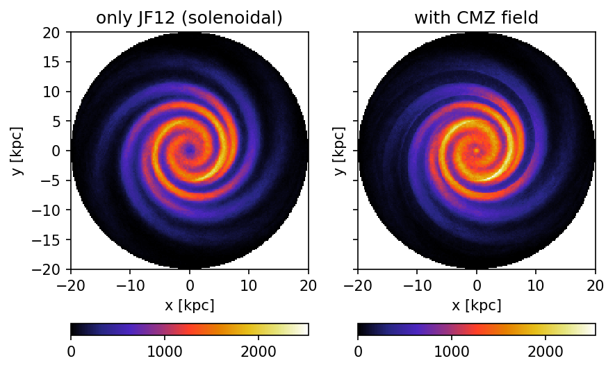
Face-on view of the Milky Way.

In the paper more bins are used. The reduction of bins here is due to the lower number of propagated candidates.

bins = np.linspace(-20, 20, 201) # In the paper 300 bins are used # np.linspace(-20, 20, 301)
binMid = (bins[1:] + bins[:-1])/2

nJF12 = np.histogram2d(data_jf12[abs(data_jf12.Z) < 0.3].X, data_jf12[abs(data_jf12.Z) < 0.3].Y, bins = [bins, bins])[0].T
nCMZ = np.histogram2d(data_cmz[abs(data_cmz.Z) < 0.3].X, data_cmz[abs(data_cmz.Z) < 0.3].Y, bins = [bins, bins])[0].T

# restrict to simulaiton volume
vmax = np.max([nJF12.max(), nCMZ.max()])
mXY, mYX = np.meshgrid(binMid, binMid)
boolR = ((mXY**2 + mYX**2) > 20**2)
nJF12[boolR] = np.nan
nCMZ[boolR] = np.nan

fig, (ax1, ax2) = plt.subplots(1,2, sharex=True, sharey=True, dpi = 150)

p1 = ax1.pcolormesh(binMid, binMid, nJF12, cmap = plt.cm.CMRmap, vmax=vmax)
ax1.set_title("only JF12 (solenoidal)")

p2 = ax2.pcolormesh(binMid, binMid, nCMZ, cmap = plt.cm.CMRmap, vmax=vmax)
ax2.set_title("with CMZ field")

for ax in (ax1, ax2):
    ax.set_aspect("equal")
    ax.set_xlabel("x [kpc]")
    ax.set_ylabel("y [kpc]")

plt.colorbar(p1, orientation = "horizontal", ax = ax1)
plt.colorbar(p2, orientation = "horizontal", ax = ax2)

fig.tight_layout()
plt.show()

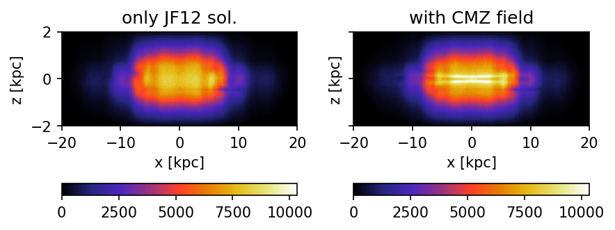
Edge-on view of the Milky Way

Additional plot of a edge on view of the Milky Way. Here, all data are integrated over the y-axis.

binsZ = np.linspace(-2, 2, 101)
binMidZ = (binsZ[1:] + binsZ[:-1])/2

nJF12 = np.histogram2d(data_jf12.X, data_jf12.Z, bins = [bins, binsZ])[0].T
nCMZ = np.histogram2d(data_cmz.X, data_cmz.Z, bins = [bins, binsZ])[0].T

vmax = np.max([nJF12.max(), nCMZ.max()])

fig, (ax1, ax2) = plt.subplots(1,2, sharex=True, sharey=True, dpi = 150)

p1 = ax1.pcolormesh(bins, binsZ, nJF12, cmap = plt.cm.CMRmap, vmax=vmax)
ax1.set_title("only JF12 sol.")

p2 = ax2.pcolormesh(bins, binsZ, nCMZ, cmap = plt.cm.CMRmap, vmax=vmax)
ax2.set_title("with CMZ field")

for ax in (ax1, ax2):
    ax.set_aspect(4)
    ax.set_xlabel("x [kpc]")
    ax.set_ylabel("z [kpc]")

plt.colorbar(p1, orientation = "horizontal", ax = ax1)
plt.colorbar(p2, orientation = "horizontal", ax = ax2)

fig.tight_layout()
plt.show()

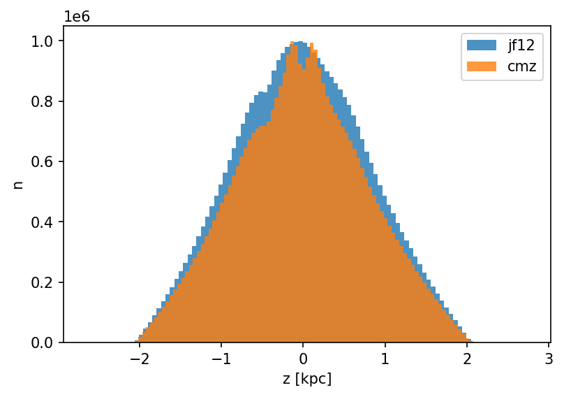
Distribution along the z-axis

Additional plot showing the distribution over the z-axis.

plt.figure(dpi = 150)
plt.hist(data_jf12.Z, bins = 100, alpha = .8, label="jf12")
plt.hist(data_cmz.Z, bins = 100, label="cmz", alpha = .8)
plt.xlabel("z [kpc]")
plt.ylabel("n")
plt.legend()
plt.show()