Example of grid based densities of the Milky Way and sampling source position

from crpropa import *
import numpy as np
import matplotlib.pyplot as plt # optional for plotting
import matplotlib as mpl

from tqdm import trange # progressbar # alternative trange = range

In this example a mass distribution is loaded from a given grid and used for the sampling of the source position of the candidates. Here, we use the H2 distribution from Mertsch & Vittino A&A 655, A64 (2021). The original data can be found here and have been converted to an CRPropa compatible format. The final data can be downloaded from the additional rescources. We use the the Model SBM15.

load grid

data_path = "/home/home1/jdo/H2-Data/Mertsch2020/H2_dens_mean_BEG03.txt" # has to be adjusted after download

origin = Vector3d(-15.96875, -15.96875, -0.46875) * kpc
nX, nY, nZ = 512, 512, 16
spacing = 0.0625 * kpc
grid = Grid1f(origin, nX, nY, nZ, spacing)
grid.setClipVolume(True) # return 0 outside of the volume

# load data
loadGridFromTxt(grid, data_path)

convert grid into a CRPropa mass distribution

isHI = False
isH2 = True
isHII = False
dens = DensityGrid(grid, isHI, isHII, isH2)
print(dens.getIsForHI(), dens.getIsForHII(), dens.getIsForH2())

False False True

(optional) plotting

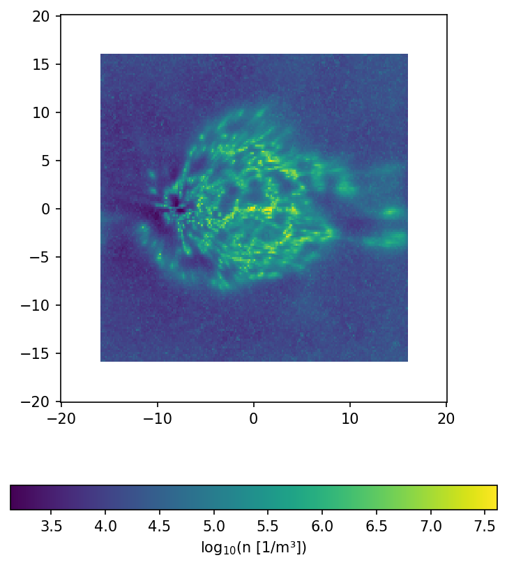
# xy plane
xRange = np.linspace(-20, 20, 250)
yRange = np.linspace(-20, 20, 200)
zRange = np.linspace(-1, 1, 150)

## xy Plane -----------------------------------------------------------
dens_data = np.zeros((len(xRange), len(yRange)))
for iX, x in enumerate(xRange):
    for iY, y in enumerate(yRange):
        dens_data[iX, iY] = dens.getDensity(Vector3d(x,y,0)*kpc)


fig, ax = plt.subplots(dpi = 150, figsize=(6,7))

ax.set_aspect("equal")
p = ax.pcolormesh(xRange, yRange, np.log10(dens_data).T)

fig.colorbar(p, label="log$_{10}$(n [1/m³])", orientation = "horizontal")
plt.show()

/tmp/ipykernel_188985/463811823.py:16: RuntimeWarning: divide by zero encountered in log10
  p = ax.pcolormesh(xRange, yRange, np.log10(dens_data).T)

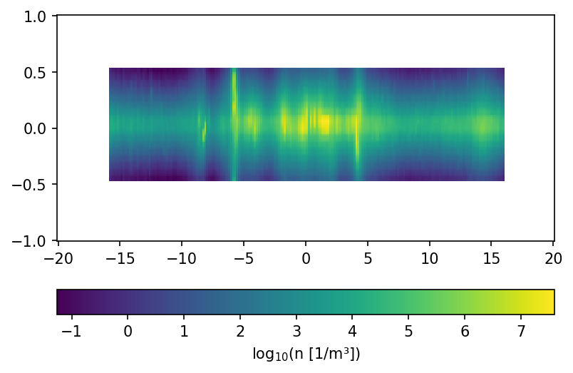
## xz Plane -----------------------------------------------------------
dens_data = np.zeros((len(xRange), len(zRange)))
for iX, x in enumerate(xRange):
    for iZ, z in enumerate(zRange):
        dens_data[iX, iZ] = dens.getDensity(Vector3d(x,0, z)*kpc)


fig, ax = plt.subplots(dpi = 150)
p = ax.pcolormesh(xRange, zRange, np.log10(dens_data).T)
fig.colorbar(p, orientation="horizontal", label="log$_{10}$(n [1/m³])")

plt.show()

/tmp/ipykernel_188985/2125385323.py:9: RuntimeWarning: divide by zero encountered in log10
  p = ax.pcolormesh(xRange, zRange, np.log10(dens_data).T)

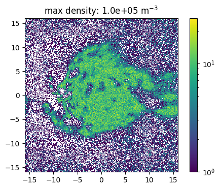
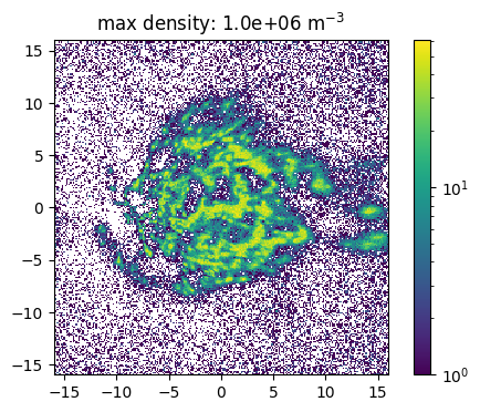
use a massdistribution as indicator for the spacial source distribution

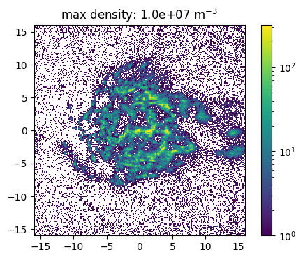
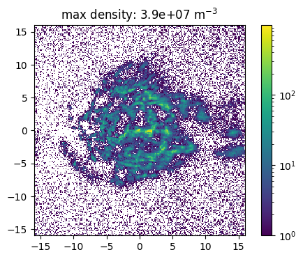
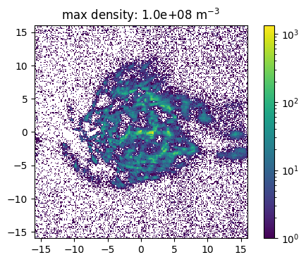
The source feature SourceMassDistribution assumes that the distribution of the source positions follows the mass distribution. To sample the position the range in which the source is sampled and the maximal density in this volume has to be set. In the following example the impact of a (non correct) maximal density is show. Here one has also to denote, that a much to high estimated maximal density leads to a raising number of tries for the sampling. This leads to larger simulation times and the maimal number of tries has to be increesed by the user.

def sample_and_plot(maxDens = 1e6, maxTries =int(1e4)):
    s = Source()
    sourceFeature = SourceMassDistribution(dens, maxDens)
    sourceFeature.setXrange(-16*kpc, 16*kpc)
    sourceFeature.setYrange(-16*kpc, 16*kpc)
    sourceFeature.setZrange(-0.5*kpc, 0.5*kpc)
    sourceFeature.setMaximalTries(int(maxTries))
    s.add(sourceFeature)

    positions = []
    for i in trange(int(5e5)):
        pos = s.getCandidate().source.getPosition()
        if(abs(pos.z) < 50 * pc):
            positions.append((pos.x, pos.y))

    positions = np.array(positions, dtype=[("X",float),("Y",float)])

    # crosscheck with plotting

    fig, ax = plt.subplots(dpi = 100)
    ax.set_aspect("equal")

    n_bin = 250
    p = ax.hist2d(positions["X"]/kpc, positions["Y"]/kpc, bins=n_bin, norm = mpl.colors.LogNorm())
    plt.title("max density: {:.1e}".format(maxDens) + " m$^{-3}$")
    fig.colorbar(p[-1])
    plt.show()

sample_and_plot(1e5)
sample_and_plot(1e6)
sample_and_plot(1e7)
sample_and_plot(np.max(dens_data), 1e5)
sample_and_plot(1e8, 1e5)

100%|██████████| 500000/500000 [00:01<00:00, 269913.01it/s]

100%|██████████| 500000/500000 [00:05<00:00, 97611.51it/s]

100%|██████████| 500000/500000 [00:28<00:00, 17340.96it/s]

100%|██████████| 500000/500000 [01:46<00:00, 4710.43it/s]

100%|██████████| 500000/500000 [04:29<00:00, 1857.67it/s]