Example for the implemented gass density distributions of the Milky Way

The following example shows the use of density distribution for the Milky Way and gives some figures of the distribution.

Currently implemented models are * Ferrière: contains HI, HII, H2; in two regions (\(R <3kpc\): arXiv:astro-ph/0702532 ; \(R >3kpc\): ApJ 497:759) * Cordes: contains HII (Nature volume 354, pages 121–124) * Nakanishi: contains HI (arXiv:astro-ph/0304338) and H2 (arXiv:astro-ph/0610769), implemented fit in (arXiv:1607.07886 Appendix C)

from crpropa import *
import numpy as np
import matplotlib.pyplot as plt

# define densities
FER = Ferriere()
NAK = Nakanishi()
COR = Cordes()

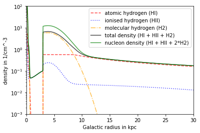
Model Ferrière

Contains HI, HII and H2 All types can be deactivated individually, e.g. FER.setisforHX() Dependency in inner Region: x,y,z Dependency in outer Region: R,z

R = np.linspace(0,30*kpc,1000)
phi = np.linspace(0,2*np.pi,360)

n_FER_HI = np.zeros((R.shape[0],phi.shape[0]))
n_FER_HII = np.zeros((R.shape[0],phi.shape[0]))
n_FER_H2 = np.zeros((R.shape[0],phi.shape[0]))
n_FER_tot = np.zeros((R.shape[0],phi.shape[0]))
n_FER_nucl = np.zeros((R.shape[0],phi.shape[0]))

# get densities
pos = Vector3d(0.)
for ir, r in enumerate(R):
    for ip, p in enumerate(phi):
        pos.x = r*np.cos(p)
        pos.y = r*np.sin(p)
        n_FER_HI[ir,ip]=FER.getHIDensity(pos)
        n_FER_HII[ir,ip]=FER.getHIIDensity(pos)
        n_FER_H2[ir,ip]=FER.getH2Density(pos)
        n_FER_tot[ir,ip]=FER.getDensity(pos)
        n_FER_nucl[ir,ip]=FER.getNucleonDensity(pos)

# plot radial
plt.figure()

plt.plot(R/kpc, n_FER_HI.mean(axis=1)*ccm, linestyle = '--',alpha = .7, color='red', label= 'atomic hydrogen (HI)')
plt.plot(R/kpc, n_FER_HII.mean(axis=1)*ccm, linestyle = ':',alpha = .7, color='blue', label = 'ionised hydrogen (HII)')
plt.plot(R/kpc, n_FER_H2.mean(axis=1)*ccm, linestyle = '-.',alpha = .7, color='orange', label= 'molecular hydrogen (H2)')
plt.plot(R/kpc, n_FER_tot.mean(axis=1)*ccm, color = 'black',alpha = .7, label = 'total density (HI + HII + H2)')
plt.plot(R/kpc, n_FER_nucl.mean(axis=1)*ccm, color ='green',alpha = .7, label = 'nucleon density (HI + HII + 2*H2)')

plt.xlabel('Galactic radius in kpc')
plt.ylabel('density in 1/cm^-3')
plt.yscale('log')
plt.axis([0,30,10**-3,10**2])
plt.legend()
plt.show()

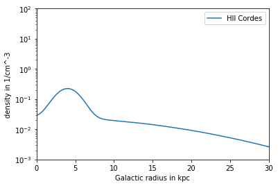
Model Cordes

Contains HII component (can not be deactivated) HIIDensity, Density and NucleonDensity are the same Dependency: R,z

n_COR_R= np.zeros(R.shape)

pos = Vector3d(0.)
for ir, r in enumerate(R):
    pos.x = r
    n_COR_R[ir]= COR.getDensity(pos)

plt.figure()
plt.plot(R/kpc, n_COR_R*ccm, label = 'HII Cordes')

plt.xlabel('Galactic radius in kpc')
plt.ylabel('density in 1/cm^-3')
plt.yscale('log')
plt.axis([0,30,10**-3,10**2])
plt.legend()
plt.show()

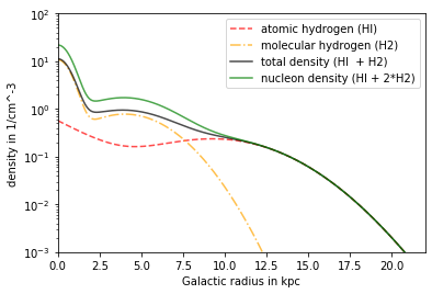
Model Nakanishi

Contains HI and H2 Both parts can be deactivated, e.g. setisforHX Dependency: R,z

n_NAK_HI = np.zeros(R.shape)
n_NAK_H2 = np.zeros(R.shape)
n_NAK_tot = np.zeros(R.shape)
n_NAK_nucl= np.zeros(R.shape)

pos = Vector3d(0.)

for ir, r in enumerate(R):
    pos.x=r
    n_NAK_HI[ir]=NAK.getHIDensity(pos)
    n_NAK_H2[ir]=NAK.getH2Density(pos)
    n_NAK_tot[ir]=NAK.getDensity(pos)
    n_NAK_nucl[ir]=NAK.getNucleonDensity(pos)

# plot radial
plt.figure()

plt.plot(R/kpc, n_NAK_HI*ccm, linestyle = '--',alpha = .7, color='red', label= 'atomic hydrogen (HI)')
plt.plot(R/kpc, n_NAK_H2*ccm, linestyle = '-.',alpha = .7, color='orange', label= 'molecular hydrogen (H2)')
plt.plot(R/kpc, n_NAK_tot*ccm, color = 'black',alpha = .7, label = 'total density (HI  + H2)')
plt.plot(R/kpc, n_NAK_nucl*ccm, color ='green',alpha = .7, label = 'nucleon density (HI + 2*H2)')

plt.xlabel('Galactic radius in kpc')
plt.ylabel('density in 1/cm^-3')
plt.yscale('log')
plt.axis([0,22,10**-3,10**2])
plt.legend()
plt.show()

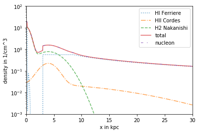
Advanced use of DensityList

For example, to combine the HI Component from Ferriere, the HII Component from Cordes and the H2 from Nakanishi

DL = DensityList()

FER.setIsForHII(False)
FER.setIsForH2(False)
DL.addDensity(FER) #only the active HI is added

DL.addDensity(COR) # only the activ HII is added, contains no other typ

NAK.setIsForHI(False)
DL.addDensity(NAK)

# plot types and sum of densities (along x-axis)

n_DL_nucl = np.zeros(R.shape)
n_DL_tot = np.zeros(R.shape)

pos = Vector3d(0.)
for ir, r in enumerate(R):
    pos.x = r
    n_DL_tot[ir] = DL.getDensity(pos)
    n_DL_nucl[ir] = DL.getDensity(pos)

plt.figure()
plt.plot(R/kpc, n_FER_HI[:,0]*ccm, label= 'HI Ferriere', linestyle =':',alpha = .7)
plt.plot(R/kpc, n_COR_R*ccm, label = 'HII Cordes', linestyle ='-.',alpha = .7)
plt.plot(R/kpc, n_NAK_H2*ccm, label='H2 Nakanishi', linestyle = '--', alpha = .7)
plt.plot(R/kpc, n_DL_tot*ccm, label= 'total', linestyle='-',alpha = .7)
plt.plot(R/kpc, n_DL_nucl*ccm, label ='nucleon', linestyle = (0, (3, 5, 1, 5, 1, 5)), alpha = .7)

plt.yscale('log')
plt.xlabel('x in kpc')
plt.ylabel('density in 1/cm^3')
plt.axis([0,30,10**-3,100])
plt.legend()
plt.show()